
Topological Data Analysis for CAN Decoding


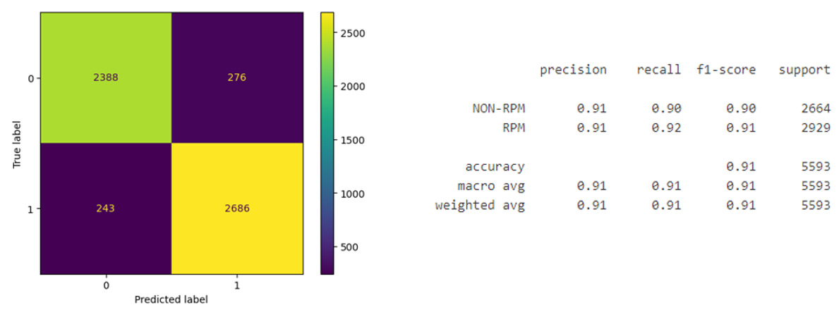
In this blog post, we have tried to explore topological data analysis in the automobile domain. Our analysis was to decode the CAN ID from the data byte on a CAN bus. Multiple methodology was explored and ultimately, a Kepler mapper an exploratory data analysis tool from TDA helped us to cluster the data. Topological features generated using persistence entropy, Betti curve and persistence image helped us to build a classifier for around 83% for 3 class and 90% for Engine RPM vs Non-RPM class.
Introduction
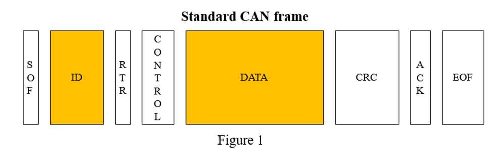
The Controller Area Network (CAN) is a communication protocol in the automotive industry that allow various components within a vehicle to exchange data efficiently on CAN BUS or CAN network. CAN data is typically transmitted on CAN BUS in the form of CAN frame. Each CAN frame [figure 1][Ref1] has an identifier or ID for a particular signal ,for example vehicle speed can have ID 11, engine rpm can have ID 23. Other relevant field for us in the study is DATA field which carry the actual information for example speed equal to 70 mph or rpm 2000. So for speed message on CAN bus could be ID : 11 , DATA 70.As of now for our analysis remaining Fields SOF, CRC are not relevant.
Decoding CAN ID via interpreting DATA frame involves classification of DATA field to identify CAN ID and finding start and stop bit in DATA field correctly to get the data value for respective CAN ID. In modern vehicles with numerous CAN buses and a wide array of sensors and control units it can be challenging. We tried to break CAN decoder in to two phases:
- Phase 1: Focused on decoding CAN ID
- Phase 2: Finding start and stop bit in DATA byte. In this study most of work is focused on phase 1.
To make a classifier on CAN DATA field we began by applying Convolutional Neural Network (CNN) techniques to raw CAN data, transforming it into a high-dimensional feature map with dimensions of 716 and for every signal of 100 timestamp generating a feature map of 100 * 716. These CNN features captured the complex patterns and relationships within the data, providing a foundation for subsequent analysis. Detail explanation is provided in Step 1: Extracting features for CNN using Interpretive Convolutions.
Topological data analysis (TDA) is a powerful tool that basically focused on understanding shape and structure of high dimension data. High dimension data has large number of features which makes it very challenging to visualize, finding useful features and extract relevant insight from it. In relevant literature we found TDA has done generally well on high dimension data. TDA leverage concept from algebraic topology to study shape and structure to analyze high dimension data.
Why TDA?
TDA is continuously evolving, with recent development of algorithm and library such as Kepler mapper, mapper interactive, giotto-tda, gudhi has make software implementation easier. Recent development in research papers also suggest its exceptional result on high dimension data as it focus on analyzing shapes and structures encourages us to use this technique on high dimension feature map of 100 *716 generated by applying CNN on raw binary CAN data. As we are looking to create a generic CAN data decoder, we have captured CAN signal as 716 CNN features and now we want to exploit TDA to analyze shape and structure of point cloud data 100* 716. In this study to decode CAN message we tried multiple experiment, few of them with satisfactory results are:
1- Cluster identification: Using mapper algorithm we can create cluster of CAN data, which can be used to group similar data points within CAN dataset. This is helpful for grouping messages with similar characteristic or in other word similar CAN ID.
2- Feature extraction: TDA can be used to reduce the dimensionality of CAN data while preserving essential topological features. This can be particularly helpful for feature extraction, which is critical for machine learning system.
Literature review
Creating Generic CAN Decoder could be very critical for understanding vehicle behavior and diagnosing issues. However, analysis of CAN data using topological Data Analysis (TDA) remains an area less explored in existing literature search in this domain. In this literature review, due to the absence of direct TDA applications in the CAN context, we tried to highlight studies that use TDA in multiple domains and discuss the technique and methodology in below section that can be relevant to the world of CAN data analysis.
1) Network intrusion detection & use of mapper algo: Network intrusion detection using Topological Data Analysis (TDA) and algorithms like Mapper has shown great promise in cybersecurity. By applying TDA techniques to network traffic data, it becomes possible to capture the intricate topological structures of network connections, making it easier to identify anomalies and potential security breaches. These insights can be highly relevant to our problem of decoding CAN data using TDA. Just as TDA can reveal unusual patterns or anomalies in network traffic, it can help uncover irregularities in CAN bus data communication, potentially indicating sensor malfunctions or security threats. [Reference :2]
2) CAN instruction detection: [CAN data has Topological Shape] The study addresses the growing concern of cybersecurity in modern vehicles, where the manipulation of CAN signals can have serious consequences. The paper presents a novel approach to intrusion detection that leverages the geometric and topological properties of CAN data. It suggests that understanding the shape of the data can provide a robust foundation for identifying attacks that may go unnoticed by existing intrusion detection systems. [Reference :3]
TDA Overview & its relevant terminology
What is Topology data analysis
Topological data analysis (TDA) is a field of analysis focused on understanding the shape and structure of complex data. By computing topological descriptors of data, such as connected components, loops, and voids, we are better able to find hidden relationships among noisy and high dimensionality data.
TDA combines algebraic topology and other tools from pure mathematics to allow a useful study of shape of the data. High dimensionality data sets severely restricts our ability to visualize them. This is why TDA can improve our ability to illustrate and analyze this data.
Key objective of TDA is to look about the shape of data.
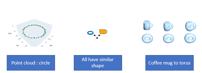
The fundamental assumption in topology is that connectivity is more important than distance.
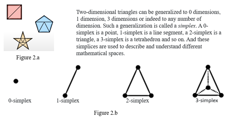
Simplices
In geometry any polygon can be formed with a combination of multiple triangles as in Figure 2.a. Now to generalize this concept in multidimension data, Triangles can be generalized to 0 dimensions, 1,2 3 dimensions or indeed to any number of dimensions. Such a generalization is called a simplex. A 0-simplex is a point, 1-simplex is a line segment, a 2-simplex is a triangle, a 3-simplex is a tetrahedron and so on. And these simplices are used to describe and understand different mathematical spaces.
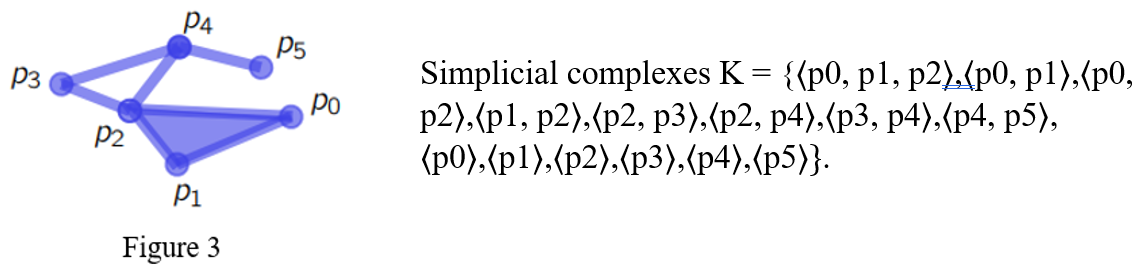
Simplicial complexes
These are used to study the property of space, by decomposing a space into [simpler pieces] simplices and then studying how these simplices are glued together.
A simplicial complex K [Reference 4] is a collection of simplices such that.
- If K contains a simplex σ, then K also contains every face of σ.
- If two simplices in K intersect, then their intersection is a face of each of them.
Rips Complex
Rip complex is constructed by taking a set of points in a metric space and connecting any pair of points whose distance is less than a fixed value known as the "radius" or “threshold”. By constructing a rip complex based on the pairwise distances between data points, it is possible to identify topological features such as clusters, voids, and tunnels that are not readily apparent from the raw data.
Homology
Homology refers to a class of methods using simplicial complexes to study topologies, it is way to measure number & type of holes in space. Some mathematicians define homology as “counting” or “detecting” holes in a varying dimension. A hole in a mathematical object is a topological structure which prevents the object from being continuously shrunk to a point.
Example to understand rips complex and homology
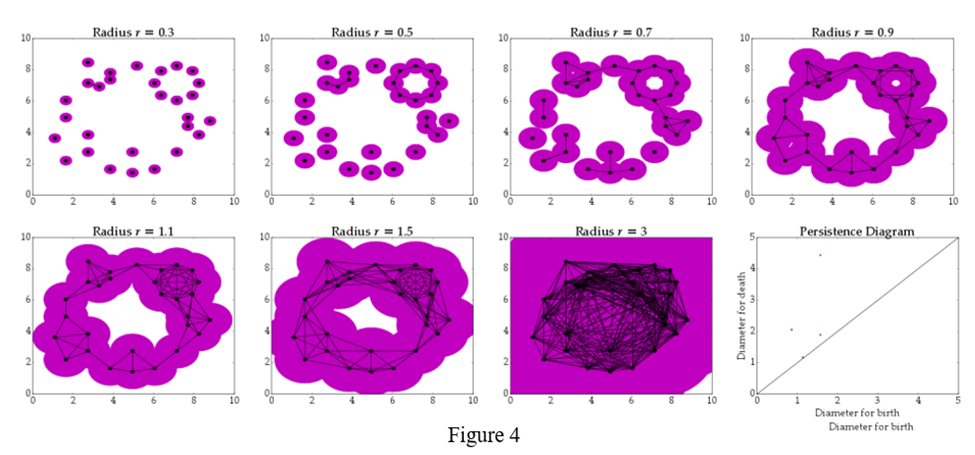
To understand rips complex and homology look at the above example [Reference 5]. Where we have multiple points, if we take pairwise Euclidean distance for all of them and if distance is less than threshold, we can say these points are connected [these will be rip complexes]. Now we can increase the threshold in other iteration to see what the connected points are:
- At radius .5 we can see one circular shape getting generated[birth], and it persist till radius .9[death], at same radius bigger circle gets generated[birth] and last till radius 1.5[death].
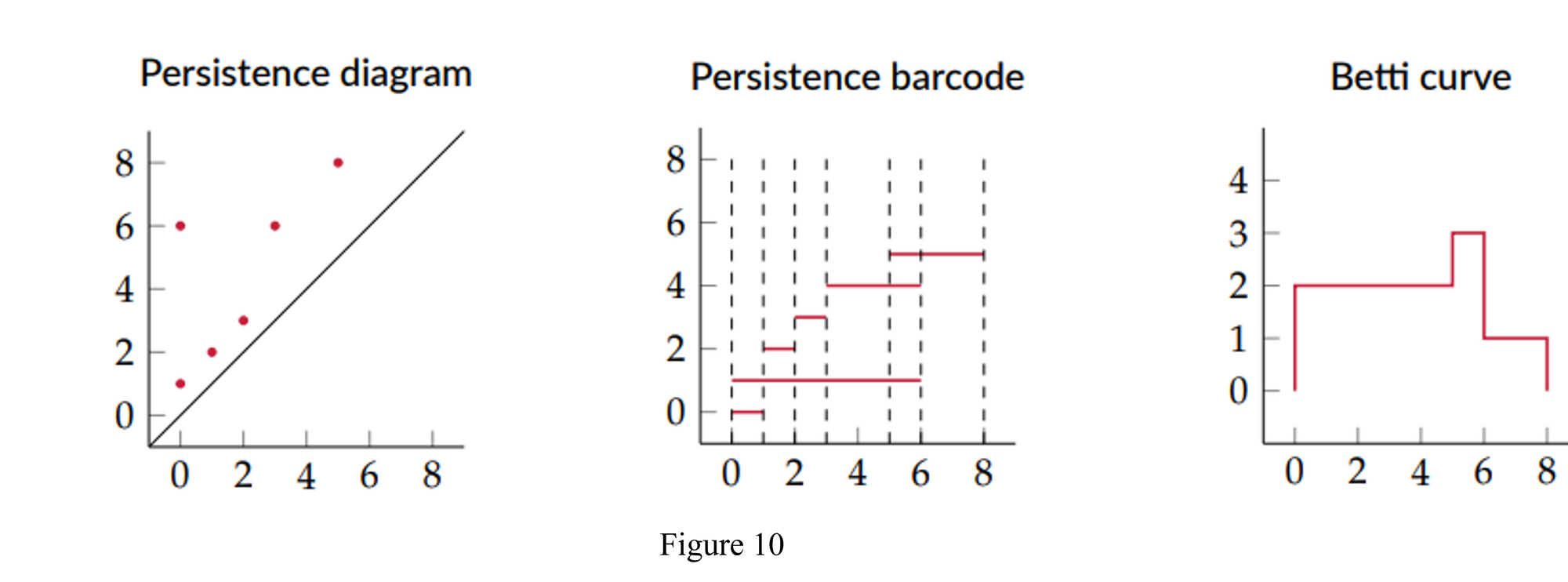
- This birth and death of topological features can be seen in persistence diagram.
Mapper algorithm
The mapper algorithm is a popular tool from topological data analysis for extracting topological summaries of high-dimensional datasets. High level flow of mapper algorithm is shown below [Reference 6], for a given point cloud step wise functioning of mapper algorithm is explain below:
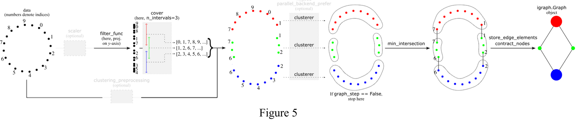
Step 1: Filter function map high dimension data set into lower dimension dataset, capturing the essential feature of dataset, it can be derived from properties of data or from domain.
Step 2: Covering function will create an overlapped partition of the lower dimension dataset generated by filter function. It will create subset of data which has some overlap with each other. In above figure, we can see points [0,1,7,8,9] all got red color and as they all are in same red color interval, number of intervals is used to create multiple partition of dataset. The more the interval gets finer and smaller details can be captured and increasing overlap will increase the connectivity among the cluster.
Step 3: Clustering algorithm such as kmean, DBSCAN can be applied to the datapoint in each interval. Each cluster will correspond the node in the graph.
Step 4: Graph will be created where nodes will represent cluster and edge will correspond to the overlapping data points.
Example of a mapper computed on double torus
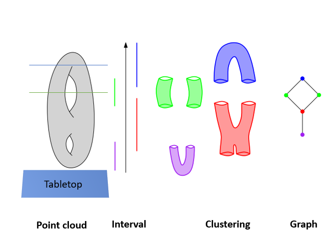
To understand how the graph is generated for a double torus[Reference 7]:
1) Let’s assume this torus is placed on a table focusing axis of two holes parallel to tabletop surface.
2) For the filter function, we can assume as height function, we are cutting torus at a height in blue interval and all the points in this subset will have the blue color. The surface created by points in this subset will have 1 connected component and any clustering algorithm will probably generate 1 cluster.
3) When we cut the same torus below at green interval, the surface that will be generated will have 2 connected component and any clustering algorithm will probably generate 2 clusters.
4) In final graph every node represents cluster and edges as overlap region.
Methodology: From CNN Features to Topological Classification
In our aim to decode the CAN data, we embarked on a journey that involved various data transformation steps, exploratory data analysis, and the utilization of Topological Data Analysis (TDA) for feature extraction and classification. Here's a detailed look at the methodological journey we undertook:
Step 0: Data collection. Data was collected from multiple brands: nearly 10 different automobile brands, with each brand contributing approximately 4 cars making it 40 vehicles data for analysis. Data logging process varied from a time frame of 1 to 3 hours.
Step 1: Extracting features for CNN using Interpretive Convolutions. CAN bus data is in hexadecimal format. For using this data to train machine learning models, it needs to be converted to decimal format. For identification of a signal all hexadecimal bits are not relevant. This relevant information is presented in labelled files with start and end bit values. But for a new CAN recording these start-end bit values are not available. Hence while converting from hexadecimal to decimal values, we use interpretive convolution approach [Ref-CANClassify]. Since we don’t know the exact bit length at priory, we use window size of multiple length and convolve around raw signal to convert it into decimal numbers. With multiple permutations of bit lengths, signs, directions we get total 716 features for a signal timesteps recording. For example, if for a particular CAN id total 20000 recordings are collected, then we get features of size 20000 x 716. For training purpose, we split these features into 100x716 arrays. [Reference: 8]
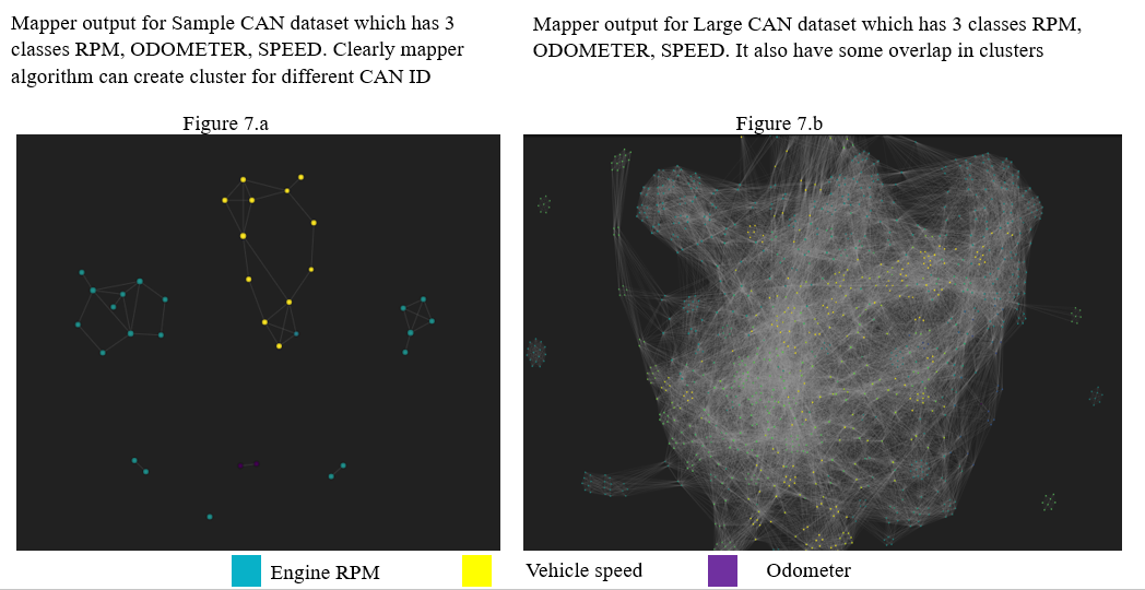
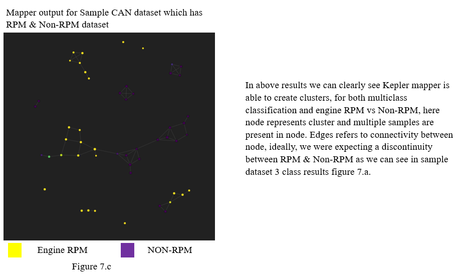
Step 2: Kepler Mapper for Exploratory Data Analysis
From our literature research, we recognize the challenges presented by high-dimensional data, and use of Kepler Mapper, a powerful tool for exploratory data analysis to tackle this. Kepler Mapper allowed us to gain insights into the data's topological structure and revealed the need for a more in-depth analysis using persistent homology.
Kepler mapper output is a graph where node represent cluster, multiple clusters are created and by doing cluster wise analysis we can find relevant feature in that cluster. This can enable us to decode start and stop bit in phase 2.
Below are some sample outputs of Kepler mapper on our CAN dataset:
Step 3: Persistent Homology
Building upon the insights gained from Kepler Mapper, we applied persistent homology to the feature map 100*716. Persistent homologies enable the identification of different homology: h0 for connected components, h1 for loop and h2 for cavities.
Step 4: Persistence Diagram and Feature Extraction
Topology of points cloud can be summarized into persistence diagram. It represents the birth and death of the homological features example H0, H1. Below figure shows sample points cloud for circle & sphere and respective persistence diagram.
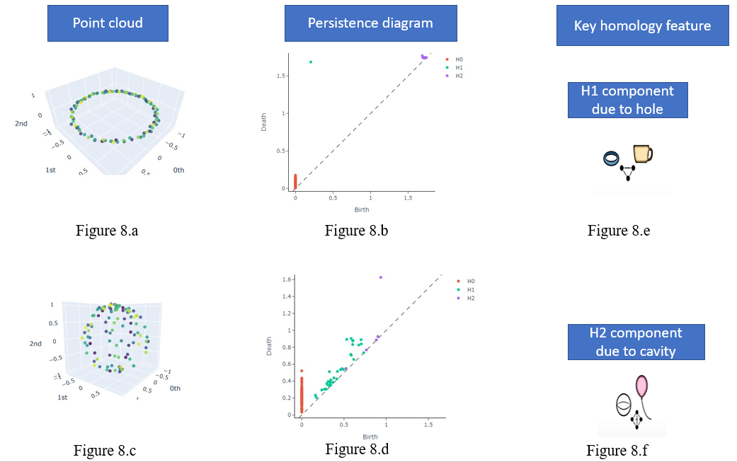
If the feature is relevant and without noise, it should be far from the diagonal.
From the machine learning application point of view topological features need to be extracted from persistence diagram using below methods
Persistence Entropy: Given a persistence diagram consisting of birth-death-dimension triples [b, d, q], sub diagrams corresponding to distinct homology dimensions are considered separately, and their respective persistence entropies are calculated as the (base 2) Shannon entropies of the collections of differences d - b (“lifetimes”), normalized by the sum of all such differences.
[Reference 9,10]
Given a filtration F = {K(t)|t ∈ R} and the corresponding persistence diagram dgm(F) = {ai = (xi , yi)| 1 ≤ i ≤ n} (being xi < yi for all i), let L = {`i = yi − xi | 1 ≤ i ≤ n}.
The persistent entropy E(F) of F is calculated as follows: E(F) = − Xn i=1 pi log(pi) where pi = `i SL , `i = yi − xi, and SL = Xn i=1 `i . Sometimes, persistent entropy E(F) will also be denoted by E(L).
Maximum persistent entropy would correspond to the situation in which all the bars in the associated persistence barcode are of equal length. Conversely, the value of the persistent entropy decreases as more bars of different lengths are present in the persistence barcode. Lower entropy means a simple shape and higher entropy means complex shapes.
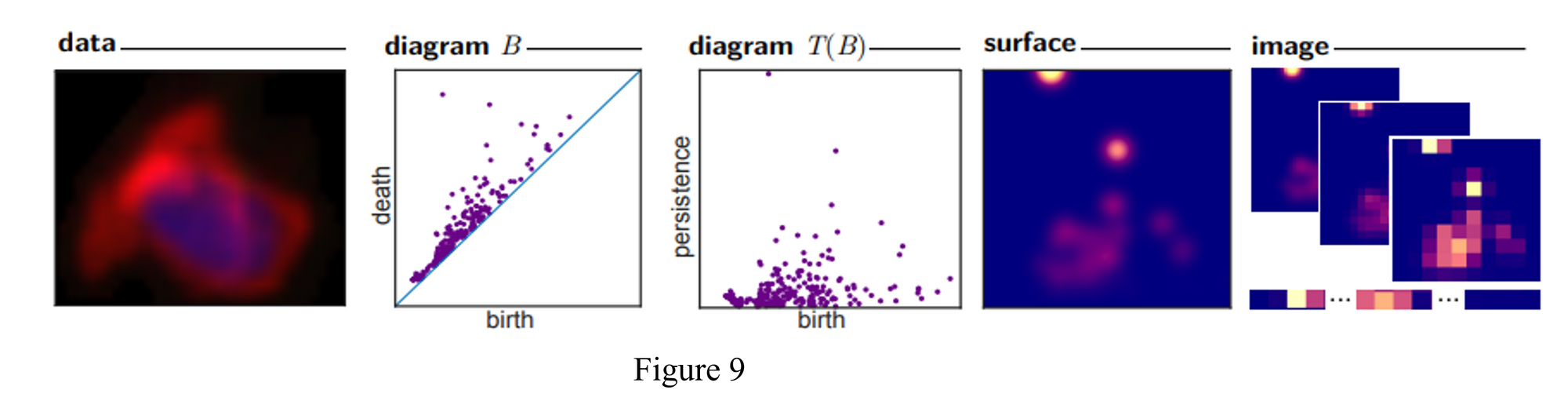
Persistence image: Persistence image [Reference 11] is a method to convert persistence diagram into a vector while maintaining an interpretable connection to the persistence diagram. Below is the pipeline that convert data to persistence image.
Betti curve: a vectorization technique that work on persistence diagram. [Reference 12]
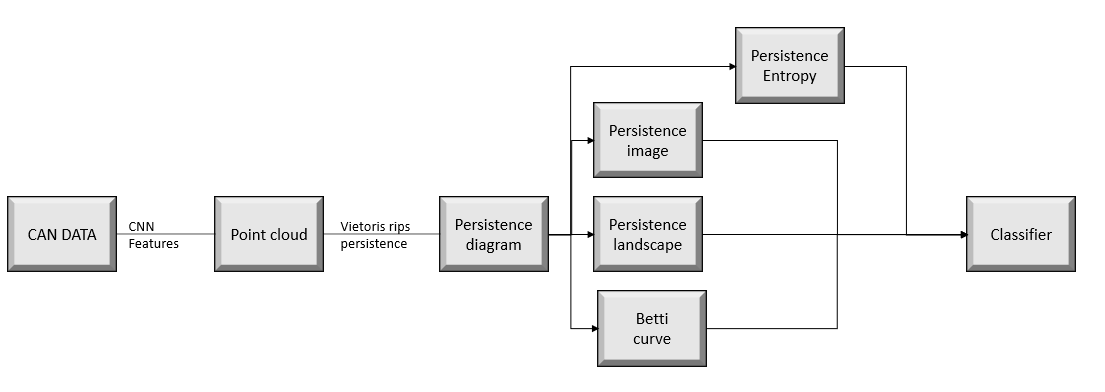
Machine learning pipeline for CAN data
High level flow of machine learning pipeline that has been implemented in experiment is shown below in figure 11. It takes raw CAN data and CNN feature map of 100 *716 generated for every signal for a time period of 100 second, topological features are generated and provided as input to the ML model:
We have also explored other approaches but as of now none were able to get satisfactory results:
1) Extracting topological features from graph but as of now didn’t get much success due to library implementation issue.
2) Treating 716 features as independent time series signal with below assumptions
- Every raw signal will have a different pattern [irrespective of scale], speed will have a different pattern than RPM and Odometer, Uniqueness of shape will not be changed based on driver & their behavior.
- Out of 716 some features should have similar topology with the original signal Ex: Difference between feature 4 persistence diagram should be minimum to original signal and major homology features should be same, also for feature 7.
Experiments & Results
Experiments should show some improvement over parallel methods for easy acceptability.
Experiment 1: Multiclass classification
In this experiment we have applied the above explained methodology, on every 100* 716 feature map. We applied VietorisRipsPersistence to extract the persistence diagram.
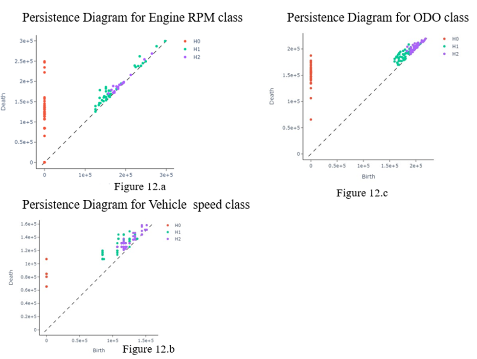
Visually we can see differentiation in persistence diagram, but clearly not one feature H0, H1, H2 is coming out as only homological feature for a class. As explained earlier multiple features like betti curve, persistence image, entropy will be calculated on top of this persistence diagram. 23 topological features are extracted for every 100 * 716 feature map and ML model is applied on these 23 features.
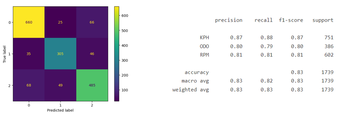
Model results: Multiclass classification
Experiment 2: Model result [ RPM vs NON-RPM]
Conclusion
CAN decoder can be a very essential tool for understanding and optimizing vehicle behavior. As TDA relies on understanding shape and structure of data, it is a novel and powerful approach to tackle the complexity of CAN data and revealing hidden structures and relationships. In our study we successfully cluster CAN data using Kepler mapper and in other approach extracted topological features which were used in ML model for classification task. As TDA continues to evolve in various domains, with our initial results it shows great promise in automotive data analysis.
In future we would like to explore more on below areas:
- Mapper algorithm using other tools like mapper interactive which supports machine learning this can enable new directions in our study.
- Every node of mapper can be explored to find out feature importance out of 716, that can lead the way to find out bit start and end phase 2.
- Extracting topological features from graph [blocked due to library implementation issue].
- Applying TDA on binary signal directly before converting it to CNN features.
ACKNOWLEDGEMENTS
We are thankful to Prof. Priyavrat Deshpande, Chennai Mathematical Institute for providing guidance to do the analysis. We would like to appreciate efforts taken by Mr. Mandar Joshi for organizing smooth content flow along with suggesting grammatical corrections in this article. We are thankful to Mr. Praneet Kuber, Mr. Kalpesh Patil, Mr. Gaurav Desai and Mr. Binit Bhagat for providing us valuable feedback on the content.
Reference
1: CAN Bus Explained - A Simple Intro [2023]
https://www.csselectronics.com/pages/can-bus-simple-intro-tutorial accessed on 4th October 2023
2: Detecting Encrypted TOR Traffic with Boosting and Topological Data Analysis
https://kepler-mapper.scikit-tda.org/en/latest/notebooks/TOR-XGB-TDA.html accessed on 4th October 2023
3: Tyree, Zachariah, Robert A. Bridges, Frank L. Combs and Michael Roy Moore. “Exploiting the Shape of CAN Data for In-Vehicle Intrusion Detection.” 2018 IEEE 88th Vehicular Technology Conference (VTC-Fall) (2018): 1-5.
4: https://www.math.uci.edu/~mathcircle/materials/MCsimplex.pdf
5: Munch, E.. “A User's Guide to Topological Data Analysis.” J. Learn. Anal. 4 (2017): n. pag.
6: van Veen et al., (2019). Kepler Mapper: A flexible Python implementation of the Mapper algorithm. Journal of Open Source Software, 4(42), 1315, https://doi.org/10.21105/joss.01315
Hendrik Jacob van Veen, Nathaniel Saul, David Eargle, & Sam W. Mangham. (2019, October 14). Kepler Mapper: A flexible Python implementation of the Mapper algorithm (Version 1.4.1). Zenodo. http://doi.org/10.5281/zenodo.4077395
7: Carrière, Mathieu, Bertrand Michel and Steve Oudot. “Statistical Analysis and Parameter Selection for Mapper.” ArXiv abs/1706.00204 (2017): n. pag.
8:Ngo, Paul, Jonathan Sprinkle and Rahul Kumar Bhadani. “CANClassify: Automated Decoding and Labeling of CAN Bus Signals.” Journal of Engineering Research and Sciences (2022): n. pag.
9: Atienza, Nieves, Rocio Gonzalez-Diaz and Matteo Rucco. “Persistent entropy for separating topological features from noise in vietoris-rips complexes.” Journal of Intelligent Information Systems 52 (2017): 637 - 655.
10: https://giotto-ai.github.io/gtda-docs/0.5.1/theory/glossary.html# accessed on 4th October 2023
11: Adams, Henry, Tegan H. Emerson, Michael J. Kirby, Rachel Neville, Chris Peterson, Patrick D. Shipman, Sofya Chepushtanova, Eric M. Hanson, Francis C. Motta and Lori Ziegelmeier. “Persistence Images: A Stable Vector Representation of Persistent Homology.” J. Mach. Learn. Res. 18 (2015): 8:1-8:35.
12:Bastian Rieck, Filip Sadlo, and Heike Leitte. “Topological Machine Learning with Persistence Indicator Functions”. In: Topological Methods in Data Analysis and Visualization V (2020), pp. 87–101. issn: 2197-666X. doi: 10.1007/978-3-030-43036-8_6. url: http://dx.doi.org/10.1007/978-3-030-43036-8_6.
13: Coffee mug to torus reference : https://en.wikipedia.org/wiki/File:Mug_and_Torus_morph.gif
You tube video for understanding:
1 : https://www.youtube.com/watch?v=5ezFcy9CIWE&list=PLzERW_Obpmv_UW7RgbZW4Ebhw87BcoXc7&index=3
2 : https://youtu.be/gVq_xXnwV-4?feature=shared
3: https://www.youtube.com/@aatrn1
4: https://www.youtube.com/@utahsoccomputationaltopolo4135/streams